In this chapter we will learn about one way to quantify the strength of a linear relationship: the covariance.
Because the covariance is a very important measure we repeatedly use throughout this course, we will first motivate where the formula comes from, and then show how to calculate it in R.
3.1 Notation
We first define some notation. We observe a sample with n observations for the variables x and y:
((x_1,y_1), (x_2,y_2), \dots, (x_n, y_n))
We will often refer to one specific observation as (x_i,y_i). This is the value of x and y for one observation (i.e. one individual/firm/market). The sample means of x and y are given by:
\bar{x}=\frac{1}{n}\sum_{i=1}^n x_i \qquad \text{ and } \qquad \bar{y}=\frac{1}{n}\sum_{i=1}^n y_i
The \sum_{i=1}^n term is mathematical notation for “take the sum over i from 1 to n”. It is defined as:
\sum_{i=1}^n x_i = x_1 + x_2 + \dots + x_n
3.2 Quadrants
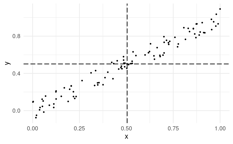
Consider again two variables x and y that have a positive linear relationship. I plot them below, adding a vertical line at \bar{x} and a horizontal line at \bar{y}:
What we can see is that most of the data points are in the top-right and bottom-left quadrants. Only a few points are in the top-left or bottom-right quadrants.
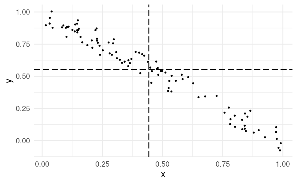
Now consider two variables that have a negative linear relationship:
What we can see here is that most of the data points are in the top-left and bottom-right quadrants. Only a few points are in the top-right or bottom-left quadrants.
From this we can conclude is that:
If most of the data points are in top right-and bottom-left quadrants, we have a positive linear relationship.
If most of the data points are in top left-and bottom-right quadrants, we have a negative linear relationship.
What we want to do with this is create a formula that captures how often we are in the top-right and bottom-left versus the top-left and bottom-right quadrants.
3.3 Towards a Formula for the Covariance: Intuition
If an observation x_i is to the right of the dashed line, then x_i-\bar{x}>0.
If an observation x_i is to the left of the dashed line, then x_i-\bar{x}<0.
If an observation y_i is above the dashed line, then y_i-\bar{y}>0.
If an observation y_i is below the dashed line, then y_i-\bar{y}<0.
We call \left( x_{i}-\bar{x} \right)\left( y_i-\bar{y} \right) the product of x_i and y_i’s deviation from their means.
If there is a positive relationship, then most points will be in the top-right and bottom-left quadrants, so \left( x_i-\bar{x} \right)\left( y_i-\bar{y} \right) will be positive for most of the observations, but could be negative for some observations. But there will be more positive terms overall and so when we sum over all observations we get:
\sum_{i=1}^n \left( x_i-\bar{x} \right)\left( y_i-\bar{y} \right)>0
If there is a negative relationship, then most points will be in the top-left and bottom-right quadrants. So \left( x_i-\bar{x} \right)\left( y_i-\bar{y} \right) will be negative for most of the observations, but could be positive for some observations. But there will be more negative terms overall and so when we sum over all observations we get:
\sum_{i=1}^n \left( x_i-\bar{x} \right)\left( y_i-\bar{y} \right)<0
Thus whether the sum \sum_{i=1}^n \left( x_i-\bar{x} \right)\left( y_i-\bar{y} \right) is positive or negative can tell us if there is a positive or a negative relationship between x and y. The covariance formula which we will introduce next is based on this sum.
3.4 Covariance Formula
The formal definition of the covariance is as follows. For two random variables X and Y, the covariance \sigma_{X,Y} is given by:
\sigma_{X,Y}=\mathbb{E}\left[\left(X-\mathbb{E}\left[X\right]\right)\left(Y-\mathbb{E}\left[Y\right]\right)\right]
where \mathbb{E}\left[X\right] is the expected value of X. In words, the covariance between two random variables is the expectation of the product of each variable’s deviation from their expected values.
With data ((x_1,y_1),\dots,(x_n,y_n)), we can estimate \sigma_{X,Y} using the sample covariance s_{X,Y}:
s_{X,Y}=\frac{1}{n-1}\sum_{i=1}^n \left( x_i-\bar{x} \right)\left( y_i-\bar{y} \right)
Notice that the sum \sum_{i=1}^n \left( x_i-\bar{x} \right)\left( y_i-\bar{y} \right) in s_{X,Y} is exactly the same as the one we saw above when analyzing the quadrants. So the covariance formula captures this idea that if the covariance is positive, then most of the points are in the top-right and bottom-left quadrants, and if the covariance is negative, then most of the points are in the top-left and bottom-right quadrants.
The only difference from above is that we divide by n-1. We do this because we are trying to estimate \sigma_{X,Y}, which is the expected value of this product of deviations from the means. We divide by n-1 instead of n because it gives less biased estimates of \sigma_{X,Y} (for the same reason we divide the sample variance by n-1).
3.5 Relationship to the Variance Formula
Let’s compare the formula for the covariance with the variance formula you learned about in Statistics 1. The formal definition of the variance is as follows. For a random variable X, the variance \sigma_X^2 is given by:
\sigma_X^2=\mathbb{E}\left[\left(X-\mathbb{E}\left[X\right]\right)^2\right]
The formula for the sample variance is given by:
s_{X}^2=\frac{1}{n-1}\sum_{i=1}^n \left( x_i-\bar{x} \right)^2
Imagine we tried to get the covariance between a variable X and itself. We replace X for Y in the covariance formula and we get:
\sigma_{X,X}=\mathbb{E}\left[\left(X-\mathbb{E}\left[X\right]\right)\left(X-\mathbb{E}\left[X\right]\right)\right]=\mathbb{E}\left[\left(X-\mathbb{E}\left[X\right]\right)^2\right]=\sigma_X^2
which is the same as the variance. We see the same if we replace y_i and \bar{y} with x_i and \bar{x} in the sample covariance formula:
s_{X,X}=\frac{1}{n-1}\sum_{i=1}^n \left( x_i-\bar{x} \right)\left( x_i-\bar{x} \right)=\frac{1}{n-1}\sum_{i=1}^n \left( x_i-\bar{x} \right)^2=s_X^2
So the covariance between a variable and itself is equal to the variance. The variance formula is a special case of the covariance formula when the two variables are the same.
3.6 Calculating the Covariance in R
We can calculate the covariance in R easily using the cov() function. We just give it two numeric vectors as arguments. Using our advertising and sales example:
We can see that the covariance is positive, indicating a positive linear relationship between advertising and sales. This is what we saw in the scatter plot.
For demonstrative purposes1, let’s try to calculate the covariance in R using the formula above instead of the built-in cov() function.
n <-nrow(df)x <- df$advertising y <- df$salesx_bar <-mean(x)y_bar <-mean(y)(1/ (n -1)) *sum((x - x_bar) * (y - y_bar))
[1] 420.9673
We get the same answer.
3.7 Interpreting the Covariance
If the covariance is positive or negative, it can tell us if the relationship is positive or not. But the size of the number we get is difficult to interpret. The covariance formula also depends on the units of the individual variables. For example, if we are interested in the covariance between height and salary, it will matter if we measure height in inches or centimeters or salary in dollars or euros.
To see this, recall that we said that advertising was in thousands of euros, and sales in millions. We can convert both variables to have units in euros as follows:
df$advertising_eur <- df$advertising *1000# convert from €1000 to € df$sales_eur <- df$sales *1000000# convert from €m to €head(df)
If we get the covariance now, we see that the scale of the number is much much larger:
cov(df$advertising_eur, df$sales_eur)
[1] 420967275126
So the covariance is heavily dependent on the units of the variables, and is difficult to tell if a covariance is large or small. It’s only able to easily tell us if the relationship is positive or negative.
What we will discuss in the next chapter is another measure of the association between two variables which doesn’t depend on the units, and is much easier to interpret the strength of the relationship. This is the correlation.
In any assessment for this course you are free to use the cov() function to calculate the covariance. We are only manually calculating the covariance here just to show that we can get the same answer that way.↩︎