In this chapter we will discuss the correlation, which is a measure of the association between two variables that is easy to interpret and does not depend on the units of the underlying variables.
4.1 Formula
The formula for the sample correlation is very similar to the covariance. The only difference is that we divide by the sample standard deviations of X and Y.
The sample correlation coefficient between X and Y is given by:
r_{X,Y}=\frac{s_{X,Y}}{s_X s_Y}
where s_{X,Y} is the covariance between X and Y (discussed in Chapter 3) and s_X and s_Y are the sample standard deviations of X and Y (the square root of the variance, which was also discussed in Chapter 3).
Dividing the covariance by the product of the sample standard deviations brings two important benefits:
The correlation coefficient must always be between -1 and +1 (this can be proven mathematically). This makes the interpretation easier, as we will see below.
The correlation coefficient has no units. If we were to change the units of X, which would scale X proportionally up or down, it would affect s_{X,Y} and s_X the same way and cancel in the formula. We will see an example of this below.
4.2 Interpretation
Similar to the covariance, if the correlation is positive, we say X and Y are positively linearly related. But we can also use how close it is to 0 or 1 to quantify the strength of the relationship:
If the correlation is high (such as 0.8), we can say “there is a strong positive linear relationship between X and Y”.
If the correlation is low (such as 0.2), we can say “there is a weak positive linear relationship between X and Y”.
If the correlation is negative, we say X and Y are negatively linearly related. We can use how close it is to 0 or -1 to quantify the strength of the relationship:
If the correlation is negative and large in magnitude (such as -0.8), we can say “there is a strong negative linear relationship between X and Y”.
If the correlation is negative but small in magnitude (such as -0.2), we can say “there is a weak negative linear relationship between X and Y”.
If the correlation is zero or very close to zero, we say “X and Y are uncorrelated”.
4.3 Perfect Linear Relationships
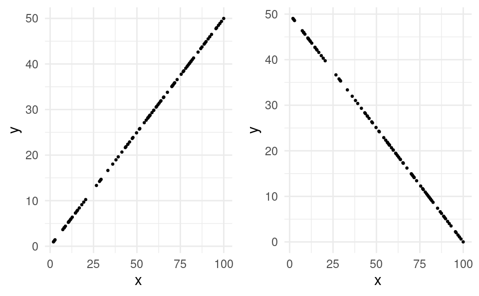
If the correlation is exactly 1, the points fall exactly along a straight upward-sloping line. This is called a perfect positive linear relationship. In this case, whenever x increases, then y always increases, and always in the same way.
If the correlation is exactly -1, the points fall exactly along a straight downward-sloping line. This is called a perfect negative linear relationship.
Here is what a scatter plot of two variables with a perfect positive linear relationship (left figure) and perfect negative linear relationship (right figure) would look like:
Sometimes x and y may be strongly related, but in a non-linear way. Because the correlation formula only measures the strength of a linear relationship, you may get a correlation of close to 0 even if x and y are clearly related.
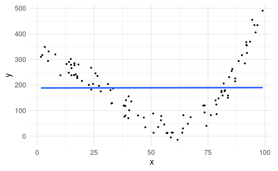
For example, suppose x and y had a U-shaped relationship, like this:
The correlation coefficient for these data points is only 0.004, very close to zero. This is despite that there is clearly a tight relationship between x and y, just not a linear one. Thus the correlation coefficient is only able to tell us about the strength of a linear relationship, and does not work for non-linear relationships. In Chapter 22 we will learn how to work with variables that are related in a non-linear way.
4.5 Calculating the Correlation in R
We can calculate the correlation in R easily using the cor() function. Very similar to the cov() function, we just give it two numeric vectors as arguments. Using our advertising and sales example:
The correlation is positive and close to 1. Thus there is a strong positive linear relationship between advertising and sales.
Let’s confirm that the correlation is unaffected by the units of the underlying variables. We convert advertising and sales to euros again and recalculate the correlation:
df <-read.csv("advertising-sales.csv")df$advertising_eur <- df$advertising *1000# convert from €1000 to € df$sales_eur <- df$sales *1000000# convert from €m to €cor(df$advertising_eur, df$sales_eur)
[1] 0.8677123
We get the same number as before. So the correlation doesn’t depend on the units.