17 Univariate Unconstrained Optimization

In Chapter 16 we learned how to make our own functions. We learned how to write a function to calculate:

f(x) = -8 -2x +x^2

The function was:

f <- function(x) {
  y <- -8 - 2 * x + x^2
  return(y)
}

In this chapter we will learn how to find the extreme point (maximum/minimum) of this univariate function (function with only one variable).

17.1 Plotting Approach

In Chapter 16, we also learned how to plot the function with ggplot(). We can get a visual view of the extreme point:

library(ggplot2)
x <- seq(from = -4, to = 6, length.out = 200)
df <- data.frame(x, y = f(x))
ggplot(df, aes(x, y)) +
  geom_line()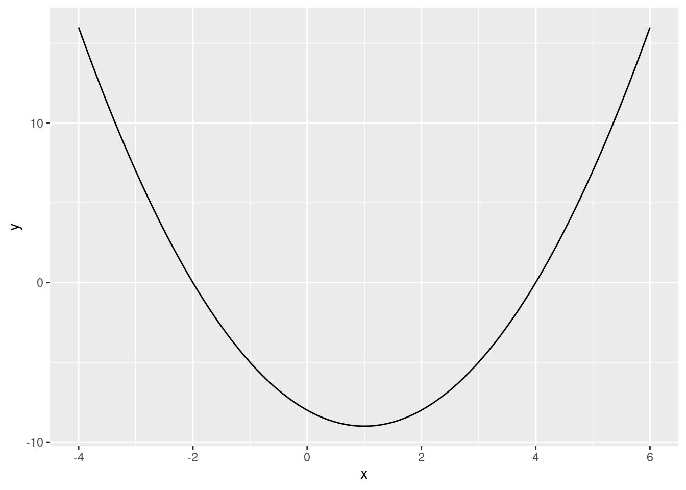

From the plot we can see the following that the function achieves a minimum at x=1.

17.2 Analytic Solution

We could have found this number analytically using calculus. Let’s do that before doing it in R. The first derivative of the function is:

f^\prime(x) = -2 + 2x To find the extreme point of the function we find the value of x where f^\prime(x)=0. This happens when: -2 + 2x = 0 Solving for x yields x=1. To see if this is a maximum or a minimum we check the second derivative: f^{\prime\prime}(x) = +2 This is positive, so we know it is a minimum. A minimum at x=1 is exactly what we see in the plot.

17.3 Using Optimization

We will now use R to find the extreme point using optimization. We can use the optimize() function to find the minimum of a univariate function in R. To do that we need to first specify the function we want to minimize and an interval to search over. We specify the interval as a vector with two elements, the lower bound and the upper bound. We will use a wide interval of [-100,+100]. We also need to specify if we are looking for a maximum or a minimum. We do that with the maximum option and set it to FALSE when looking for a minimum:

optimize(f, interval = c(-100, 100), maximum = FALSE)

$minimum
[1] 1

$objective
[1] -9

We can see that we get the same result as the plot and the analytic solution. The minimum value occurs at x=1 and the value of the function is -9 at that point.

If you want to maximize a function instead, we need to set maximum = TRUE.

The optimize() function returns a named list. Suppose we assign the output of the optimize() function to f_min:

f_min <- optimize(f, interval = c(-100, 100), maximum = FALSE)
class(f_min)

[1] "list"

To extract the minimum from this list we can use f_min$minimum. The $ works for extraction with named lists the same way as with dataframes. To extract the value of the function at the minimum, we can use f_min$objective:

f_min$minimum

[1] 1

f_min$objective

[1] -9

17.4 Examples from Mathematics for E&BI

17.4.1 Basic Order Quantity Model

Suppose that you run a bicycle shop. You sell d=8000 bikes per year with the sales equally spread out throughout the year. You buy the bikes from a manufacturer for p=1000 per bike and every time you place an order you need to pay c=100. You also need to pay a holding cost of h=10 per bike per year (like paying rent for storage area). Assume that you place an order for more bikes every time your inventory goes to zero.

You face the problem of determining the optimal number of bikes you should order each time your inventory goes to zero. Your objective is to choose the quantity to buy in each order q to minimize total costs TC(q):

TC(q)= \underbrace{\frac{cd}{q}}_{\substack{\text{Total} \\ \text{ordering} \\ \text{costs}}} + \underbrace{pd}_{\substack{\text{Total}\\\text{cost of}\\\text{bikes}}} + \underbrace{\frac{hq}{2}}_{\substack{\text{Total}\\\text{holding}\\\text{costs}}} Here is a summary of where these terms come from:

\frac{d}{q} is the number of times in the year that you place an order, because you sell d in total over the year and order q bikes each time you place an order. With a cost of c per order we get \frac{cd}{q} for the total ordering costs.
You sell d bikes per year and need to pay p per bike, so pd is the total costs of the bikes themselves.
Just before you order a new batch of bikes you have 0 in inventory, and just after you order you have q in inventory. So on average you have \frac{q}{2} bikes in inventory throughout the year. The holding cost is h per bike, so the total holding costs is \frac{hq}{2}.

In Mathematics for E&BI you learned that you can take the first derivative of the TC(q) function and find the value of q that solves TC^\prime(q)=0 to get the optimal order quantity. It turned out to be q=\sqrt{\frac{2cd}{h}}. With c=100, d=8000 and h=10, we get q=\sqrt{2\times 100 \times 8000 / 10}=400.

Suppose for the moment that the function TC(q) was very hard to take the derivative of, or even if you could take the derivative of it, you weren’t able to solve it for q. We could instead use R to find the optimal order quantity without taking any derivatives or doing any algebra. We can do this by creating a function which gives the total costs as a function of the order quantity q:

tc <- function(q) {
 total_costs <- c*d/q + p*d + h*q/2 
 return(total_costs)
}

If we set values for the other parameters, d, p, c and h, we can use the optimize() function to get the optimal order quantity:

d <- 8000  # total demand
p <- 1000  # price per bike
c <- 100   # ordering costs
h <- 10    # holding costs
optimize(tc, c(0, 1000))

$minimum
[1] 400.0001

$objective
[1] 8004000

We can see that we also get 400, the same answer, and we didn’t have to do any derivatives or algebra at all. Therefore you can use R to optimize functions in cases where it is difficult to do things by hand.

Note: You will notice that the answer optimize() found is 400.0001, slightly different from 400. This is because of the default accuracy setting in the optimize() function. We can get a more accurate answer by specifying a smaller tolerance level with the tol argument:

optimize(tc, c(0, 1000), tol = 0.00001)

$minimum
[1] 400

$objective
[1] 8004000