(2^4 + 10) / (8 * sqrt(4))[1] 1.625
Write an R command that calculates the following:
\frac{2^4 + 10}{8\times \sqrt{4}} Provide both the numerical answer and the R command.
(2^4 + 10) / (8 * sqrt(4))[1] 1.625Write an R command that calculates \log_2\left(64\right)
Provide both the numerical answer and the R command.
log(64, base = 2)[1] 6If we create the following vector in R, what class will it be?
c(1, 2, "c", "d")Note: You do not need to supply your code for this question.
Answer: All elements of a vector must be of the same type. If characters are present, all elements are coerced to character. We can also find the class using the class() function:
class(c(1, 2, "c", "d"))[1] "character"Write an R command that generates a numeric vector containing the following sequence:
(10, 10, 20, 20, 30, 30, 40, 40, \dots, 470, 470, 480, 480, 490, 490, 500, 500)
rep(seq(from = 10, to = 500, by = 10), each = 2) [1] 10 10 20 20 30 30 40 40 50 50 60 60 70 70 80 80 90 90
[19] 100 100 110 110 120 120 130 130 140 140 150 150 160 160 170 170 180 180
[37] 190 190 200 200 210 210 220 220 230 230 240 240 250 250 260 260 270 270
[55] 280 280 290 290 300 300 310 310 320 320 330 330 340 340 350 350 360 360
[73] 370 370 380 380 390 390 400 400 410 410 420 420 430 430 440 440 450 450
[91] 460 460 470 470 480 480 490 490 500 500The logical vectors a and b have equal length. Which of the following options is always the same as !(a | b), regardless of the contents of a and b?
!a & !b!a | !ba | bNote: You do not need to supply your code for this question.
Answer:
!a & !b
Explanation: We can make two vectors a and b that cover every possible combination of TRUE and FALSE and then compare the target output with each of the options:
a <- c(TRUE, TRUE, FALSE, FALSE)
b <- c(TRUE, FALSE, TRUE, FALSE)

# The target output is:
!(a | b)
[1] FALSE FALSE FALSE TRUE# Options
!a & !b[1] FALSE FALSE FALSE TRUE!a | !b[1] FALSE TRUE TRUE TRUEa | b[1] TRUE TRUE TRUE FALSEThe first one matches and the others don’t. The reason this first one matches is because of De Morgan’s laws which are:
The question concerns !(a | b) which is the negation of “A or B” (the 2nd law). From this we know it is the same as “not A and not B”, which is !a & !b in R, the first of the 3 multiple choice options.
Download the dataset ceosal.csv. The dataset contains information on chief executive officers (CEOs) at different companies. The variable descriptions are:
salary: CEO compensation in 1990 (in dollars).age: CEO agecollege: =1 if the CEO attended college and =0 otherwise.grad: =1 if the CEO attended post-graduate education and =0 otherwise.comten: Years the CEO worked with the company.ceoten: Years as CEO with the company.profits: Profits of the company in 1990 (in dollars).When reading the dataset into R, assign it to df.
df <- read.csv("ceosal.csv")How many observations are in the dataset?
Provide both the numerical answer and the R command required to obtain the answer (if the dataframe is assigned to df).
nrow(df)[1] 177What is the median of the variable comten?
Provide both the numerical answer and the R command required to obtain the answer (if the dataframe is assigned to df).
median(df$comten)[1] 23What is the mean salary of the CEOs that attended post-graduated education?
Provide both the numerical answer and the R command required to obtain the answer (if the dataframe is assigned to df).
mean(df$salary[df$grad == 1])[1] 864212.8How many people in the dataset attended college but didn’t attend post-graduate education?
Provide both the numerical answer and the R command required to obtain the answer (if the dataframe is assigned to df).
sum(df$college == 1 & df$grad == 0)[1] 78# Or alternatively:
sum(df$college[df$grad == 0])[1] 78In the dataset, what is the longest someone worked at a company (in years) for before they became CEO?
Provide both the numerical answer and the R command required to obtain the answer (if the dataframe is assigned to df).
max(df$comten - df$ceoten)[1] 39Download the dataset euro-dollar-2022.csv. The dataset contains the closing Euro-Dollar exchange rate (variable Price) each day throughout 2022, together with the opening, highest and lowest exchange rate. Furthermore, it includes the volume traded and the percentage daily change in the closing price.
Download the following template script and use it to clean the data and answer the questions that follow.
When reading the dataset into R, assign it to df.
You should do the following cleaning tasks to your dataframe df:
Date variable to a date.Date ascending (the earliest date in the data should be first, the most recent date last).Price, Open, High and Low to numeric.Vol to numeric. For example, "33.87K" should be 33870. Hint: First use the gsub() function to remove the K. Then convert the variable to numeric format. Finally multiply it by 1,000.Change to numeric. Tip: Use gsub("\\%", "", x) to remove a percentage symbol from x.If you did all the steps correctly, you should have 260 observations. The average of the high variable should be 0.9561. The average of the vol variable should be 79920. If only some of these match your cleaned dataset, you will still be able to answer some of the questions correctly.
# First perform all the cleaning tasks:

df <- read.csv("euro-dollar-2022.csv")

# Format the date:
head(df$Date)
[1] "12/31/22" "12/30/22" "12/29/22" "12/28/22" "12/27/22" "12/26/22"# Format is MM/DD/YY (year without century):
df$Date <- as.Date(df$Date, format = "%m/%d/%y")
# Order by date:
df <- df[order(df$Date), ]
# Drop observations with missing data:
df <- na.omit(df)
# Convert prices data to numeric:
df$Price <- as.numeric(df$Price)
df$Open <- as.numeric(df$Open)
df$High <- as.numeric(df$High)
df$Low <- as.numeric(df$Low)
# Convert volume to numeric:
df$Vol <- 1000 * as.numeric(gsub("K", "", df$Vol))
# Convert Change numeric:
df$Change <- as.numeric(gsub("\\%", "", df$Change))
# Convert variable names to lower case:
names(df) <- tolower(names(df))Create a variable called hml which is the high variable minus the low variable.
Use this variable to write an R command that computes the mean of this variable.
Assign the output of this command to the variable a11 in your script and write its numerical value in the box below.
df$hml <- df$high - df$low
a11 <- mean(df$hml)
a11
[1] 0.009504231Write an R command that computes the median of the vol variable.
Assign the output of this command to the variable a12 in your script and write its numerical value in the box below.
a12 <- median(df$vol)
a12
[1] 80185Write an R command that computes the largest negative daily price change in the data.
Assign the output of this command to the variable a13 in your script and write its numerical value (without the % symbol) in the box below.
a13 <- min(df$change)
a13
[1] -2.1Write an R command that finds the date on which the largest volume was traded.
Assign the output of this command to the variable a14 in your script and write the day, month and year in the boxes below.
a14 <- df$date[df$vol == max(df$vol)]
a14
[1] "2022-06-16"# Alternatively, sort the data by volume descending and get the first date:
df[order(df$vol, decreasing = TRUE), ]$date[1][1] "2022-06-16"The following 3 questions will involve working with the following mathematical function defined over all real numbers x:
f(x) = -x^2 + 2x - 5
Plot the function between the x values -3 and +5. Choose the answer below which best describes the shape of this function:
f <- function(x) {
  y <- -x^2 + 2*x - 5
  return(y)
}
library(ggplot2)
x <- seq(-3, 5, length.out = 2000)
y <- f(x)
df <- data.frame(x, y)
ggplot(df, aes(x, y)) + geom_line()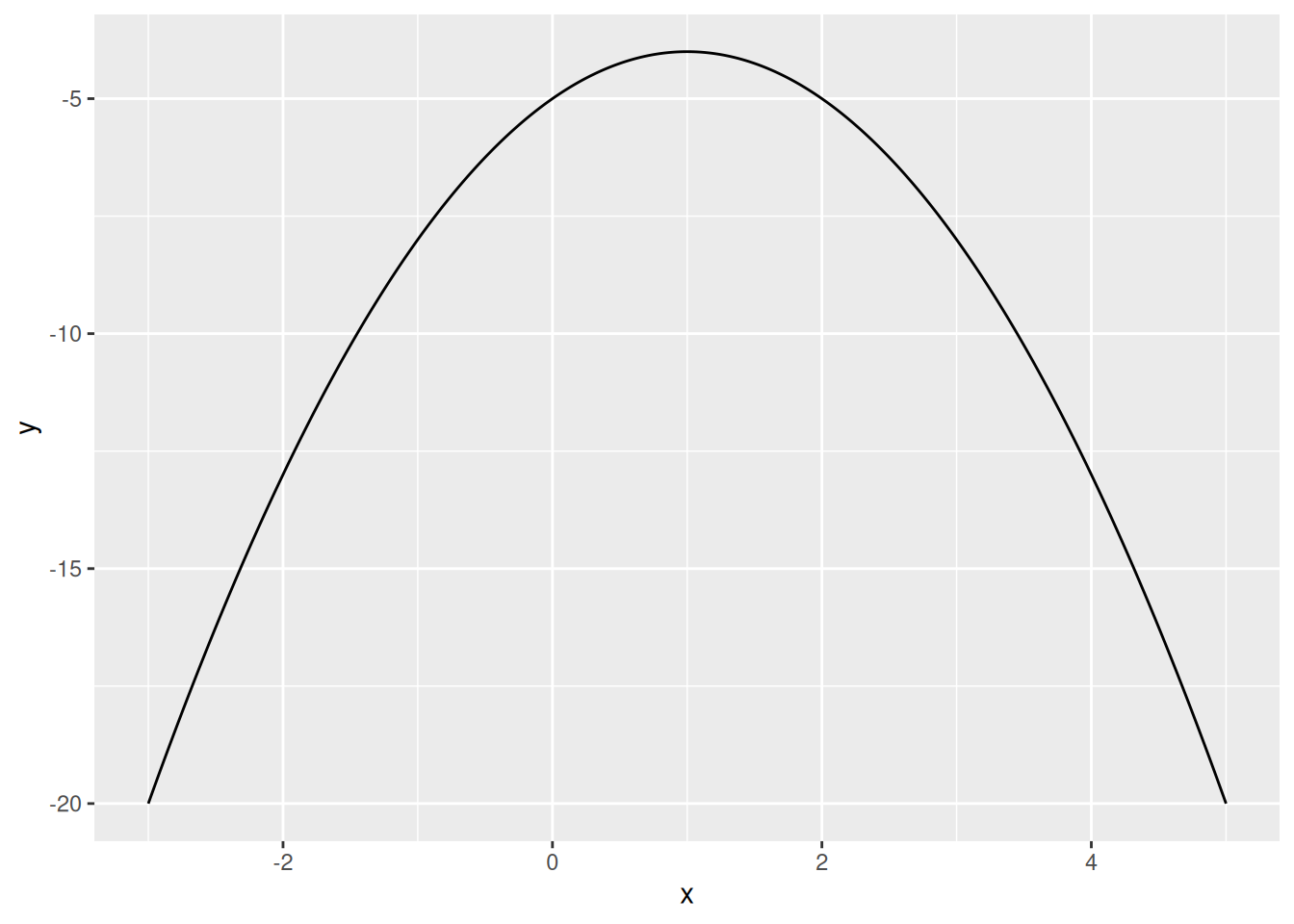
# We can see that it has an inverted U shape.Write an R command that finds the value of x that maximizes this function.
Write the numerical value of the output of this command in the box below.
f_max <- optimize(f, c(-100, 100), maximum = TRUE)
f_max$maximum
[1] 1Write an R command that finds the value of the function f(x) at its maximum value.
Write the numerical value of the output of this command in the box below.
f_max$objective[1] -4# or alternatively:
f(f_max$maximum)[1] -4Download the two datasets:
country, year and gdp_pc_growth. The variable gdp_pc_growth is the growth rate of the country’s per capita gross domestic product (GDP) in that year.country, year and lending_rate. The variable lending_rate is the lending interest rate in that country in that year.Assign the dataset gdp-per-capita-growths.csv to df1 and lending-rates.csv to df2 in your script.
Using the dataset gdp-per-capita-growths.csv, calculate the average per capita GDP growth rate across countries by year.
Write an R command that finds the year in the data when the average GDP per capita growth rate the smallest?
Write the numerical value of your answer in the box below.
df1 <- read.csv("gdp-per-capita-growths.csv")
df2 <- read.csv("lending-rates.csv")

# Find average GDP per growth growth across countries by year:
tmp <- aggregate(gdp_pc_growth ~ year, data = df1, FUN = mean)

# Sort from smallest to largest:
tmp <- tmp[order(tmp$gdp_pc_growth), ]

# Get the year with the smallest value of GDP per capita growth:
tmp$year[1]
[1] 2009Use R to merge the datasets gdp-per-capita-growths.csv and lending-rates.csv together by the variables "country" and "year", dropping observations without a match. Your merged dataset should have 2,572 observations and 4 variables.
Write an R command that computes the mean growth rate in GDP per capita in the merged dataset.
Write the numerical value of your answer in the box below.
# Merge by country and year:
df <- merge(df1, df2, by = c("country", "year"))

# Check that dimensions match the question description:
dim(df)
[1] 2572 4# Get answer:
mean(df$gdp_pc_growth)[1] 2.456217Create a subset of the merged data from Question 19 which only includes data on the Netherlands. This is when the country variable equals "Netherlands".
Reshape the Netherlands data to long format and use this long-format data to create a line plot of per capita GDP growth and the lending rate over time in the Netherlands. Choose the answer below which best describes what the plot shows in 2009:
Hint: Your long-format data for the Netherlands should have 4 variables: "country", "year", "variable" and "value", where:
"country" is "Netherlands" everywhere."year" takes on the values 2000-2013 repeated twice."variable" contains the two variable names ("gdp_pc_growth" and "lending_rate") repeated for each year."value" contains the values of those variables in those years.The first 3 rows of your reshaped data should look like:
    country year      variable      value
Netherlands 2000 gdp_pc_growth  3.4535383
Netherlands 2001 gdp_pc_growth  1.5574581
Netherlands 2002 gdp_pc_growth -0.4203677
# Create subset of merged data which only includes the Netherlands:
df_nl <- df[df$country == "Netherlands", ]
# Reshape from long to wide:
library(reshape2)
df_nl_long <- melt(df_nl, id.vars = c("country", "year"))
# Plot GDP per capita growth and lender rate over time:
library(ggplot2)
ggplot(df_nl_long, aes(year, value, color = variable)) +
geom_line()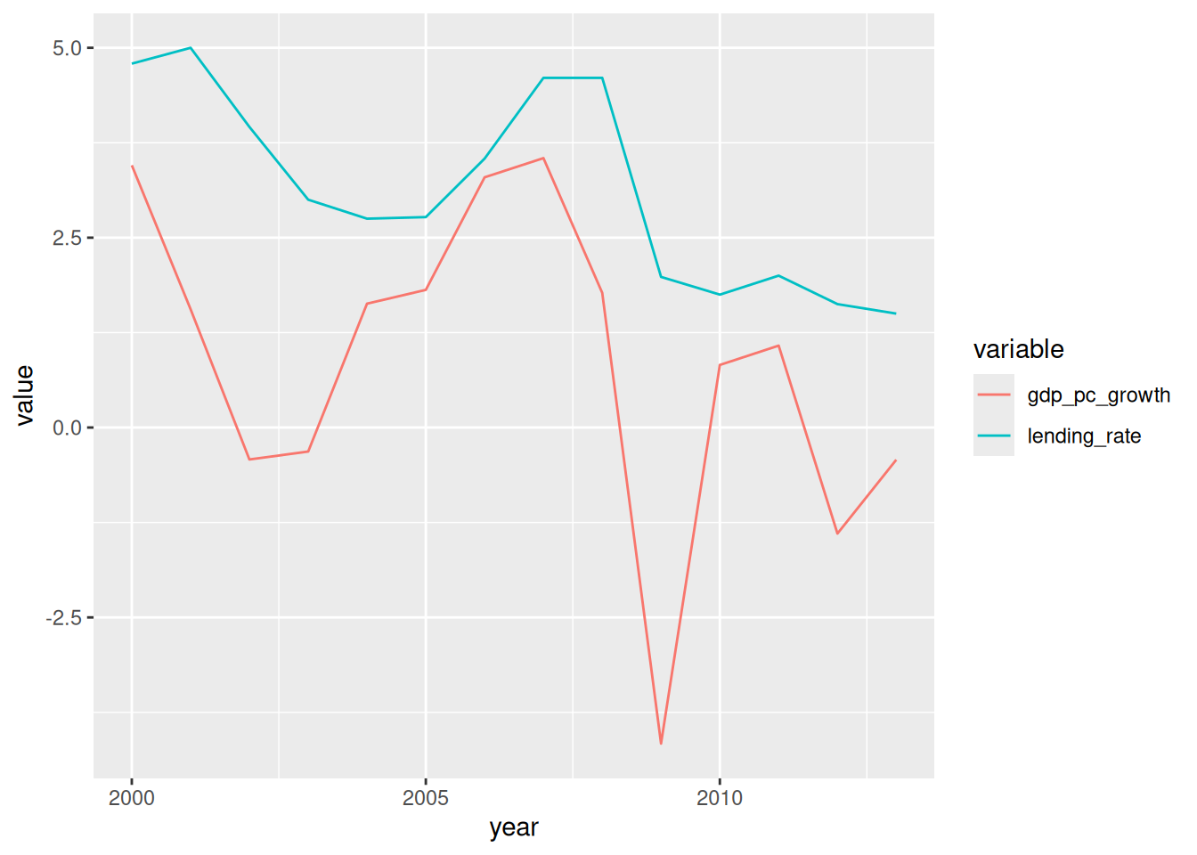
# Answer: GDP per capita growth fell sharply, and the lending rate also decreased.